2 R Markdown basics

Here is a brief introduction to using R Markdown. Markdown is a simple formatting syntax for authoring HTML, PDF, and MS Word documents and much, much more. R Markdown provides the flexibility of Markdown with the implementation of R input and output. For more details on using R Markdown see http://rmarkdown.rstudio.com.

2.1 Basic markdown syntax

2.1.1 Whitespace

Be careful with your spacing. While whitespace largely is ignored, it does at times give markdown signals as to how to proceed. As a habit, try to keep everything left aligned whenever possible, especially as you type a new paragraph. In other words, there is no need to indent basic text in the Rmd document (in fact, it might cause your text to do funny things if you do).

2.1.2 Italics and bold

• Italics are done like *this* or _this_
• Bold is done like **this** or __this__
• Bold and italics is done like ***this***, ___this___, or (the most transparent solution, in my opinion) **_this_**

2.1.3 Inline code

• Inline code is created with backticks like `this`

2.1.4 Sub and superscript

Sub₂ and super² script is created like this~2~ and this^2^

2.1.5 Strikethrough

• Strikethrough is done ~~like this~~

2.1.6 ‘Escaping’ (aka “What if I need an actual asterisk?”)

• To include an actual *, _ or \, add another \ in front of them: \*, \_, \\

2.1.7 Endash (–), emdash (—)

• – and — with -- and ---

2.1.8 Blockquotes

Do like this:

Put a > in front of the line.

2.1.9 Headings

Section headers are created with #’s of increasing number, i.e. 

• # First-level heading
• ## Second-level heading
• ### Etc.

In PDF output, a level-five heading will turn into a paragraph heading, i.e. \paragraph{My level-five heading}, which appears as bold text on the same line as the subsequent paragraph.

2.1.10 Lists

Unordered list by starting a line with an * or a -:

• Item 1
• Item 2

Ordered lists by starting a line with a number. Notice that you can mislabel the numbers and Markdown will still make the order right in the output:

1. Item 1
2. Item 2

To create a sublist, indent the values a bit (at least four spaces or a tab):

1. Item 1
2. Item 2
3. Item 3
   • Item 3a
   • Item 3b

2.1.11 Line breaks

The official Markdown way to create line breaks is by ending a line with more than two spaces.

Roses are red. Violets are blue.

This appears on the same line in the output, because we didn’t add spaces after red.

Roses are red.
Violets are blue.

This appears with a line break because I added spaces after red.

I find this is confusing, so I recommend the alternative way: Ending a line with a backslash will also create a linebreak:

Roses are red.
Violets are blue.

To create a new paragraph, you put a blank line.

Therefore, this line starts its own paragraph.

2.1.12 Hyperlinks

• This is a hyperlink created by writing the text you want turned into a clickable link in [square brackets followed by a](https://hyperlink-in-parentheses)

2.1.13 Footnotes

• Are created¹ by writing either ^[my footnote text] for supplying the footnote content inline, or something like [^a-random-footnote-label] and supplying the text elsewhere in the format shown below ²:

[^a-random-footnote-label]: This is a random test.

2.1.14 Comments

To write comments within your text that won’t actually be included in the output, use the same syntax as for writing comments in HTML. That is, <!-- this will not be included in the output -->.

2.1.15 Math

The syntax for writing math is stolen from LaTeX. To write a math expression that will be shown inline, enclose it in dollar signs. - This: $A = \pi*r^{2}$ Becomes: \(A = \pi*r^{2}\)

To write a math expression that will be shown in a block, enclose it in two dollar signs.
This: $$A = \pi*r^{2}$$

Becomes: \[A = \pi*r^{2}\]

To create numbered equations, put them in an ‘equation’ environment and give them a label with the syntax (\#eq:label), like this:

\begin{equation} 
  f\left(k\right) = \binom{n}{k} p^k\left(1-p\right)^{n-k}
  (\#eq:binom)
\end{equation} 

Becomes: \[\begin{equation} f\left(k\right)=\binom{n}{k}p^k\left(1-p\right)^{n-k} \tag{2.1} \end{equation}\]

For more (e.g. how to theorems), see e.g. the documentation on bookdown.org

2.2 Executable code chunks

The magic of R Markdown is that we can add executable code within our document to make it dynamic.

We do this either as code chunks (generally used for loading libraries and data, performing calculations, and adding images, plots, and tables), or inline code (generally used for dynamically reporting results within our text).

The syntax of a code chunk is shown in Figure 2.1.

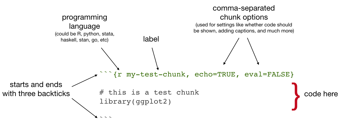
Figure 2.1: Code chunk syntax

Common chunk options include (see e.g. bookdown.org):

• echo: whether or not to display code in knitted output
• eval: whether or to to run the code in the chunk when knitting
• include: whether to include anything from the from a code chunk in the output document
• fig.cap: figure caption
• fig.scap: short figure caption, which will be used in the ‘List of Figures’ in the PDF front matter

IMPORTANT: Do not use underscoores in your chunk labels - if you do, you are likely to get an error in PDF output saying something like “! Package caption Error: \caption outside float”.

2.2.1 Setup chunks - setup, images, plots

An R Markdown document usually begins with a chunk that is used to load libraries, and to set default chunk options with knitr::opts_chunk$set.

In your thesis, this will probably happen in index.Rmd and/or as opening chunks in each of your chapters.

```{r setup, include=FALSE}
# don't show code unless we explicitly set echo = TRUE
knitr::opts_chunk$set(echo = FALSE)

library(tidyverse)
```

2.2.2 Including images

Code chunks are also used for including images, with include_graphics from the knitr package, as in Figure 2.2

knitr::include_graphics("figures/sample-content/beltcrest.png")

Figure 2.2: Oxford logo

Useful chunk options for figures include:

• out.width (use with a percentage) for setting the image size
• if you’ve got an image that gets waaay to big in your output, it will be constrained to the page width by setting out.width = "100%"

Figure rotation

You can use the chunk option out.extra to rotate images.

The syntax is different for LaTeX and HTML, so for ease we might start by assigning the right string to a variable that depends on the format you’re outputting to:

if (knitr::is_latex_output()){
  rotate180 <- "angle=180"
} else {
  rotate180 <- "style='transform:rotate(180deg);'"
}

Then you can reference that variable as the value of out.extra to rotate images, as in Figure 2.3.

Figure 2.3: Oxford logo, rotated

2.2.3 Including plots

Similarly, code chunks are used for including dynamically generated plots. You use ordinary code in R or other languages - Figure 2.4 shows a plot of the cars dataset of stopping distances for cars at various speeds (this dataset is built in to R).

cars %>% 
  ggplot() +
    aes(x = speed, y = dist) +
    geom_point()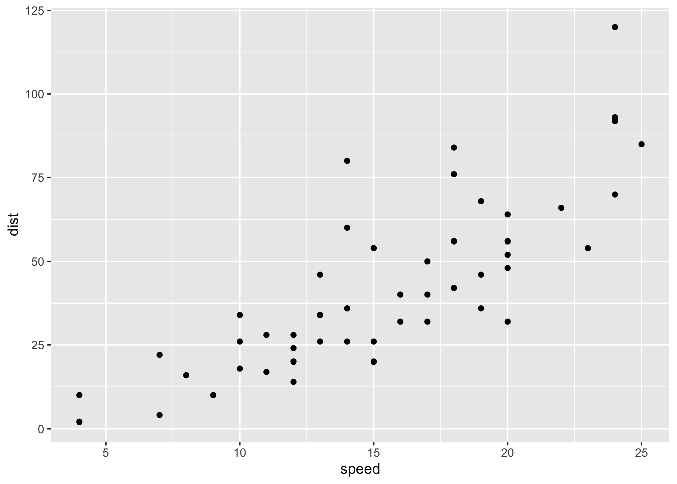

Figure 2.4: A ggplot of car stuff

Under the hood, plots are included in your document in the same way as images - when you build the book or knit a chapter, the plot is automatically generated from your code, saved as an image, then included into the output document.

2.2.4 Including tables

Tables are usually included with the kable function from the knitr package.

Table 2.1 shows the first rows of that cars data - read in your own data, then use this approach to automatically generate tables.

cars %>% 
  head() %>% 
  knitr::kable(caption = "A knitr kable table")

Table 2.1: A knitr kable table

speed	dist
4	2
4	10
7	4
7	22
8	16
9	10

• Gotcha: when using kable, captions are set inside the kable function
• The kable package is often used with the kableExtra package

2.2.5 Control positioning

One thing that may be annoying is the way R Markdown handles “floats” like tables and figures. In your PDF output, LaTeX will try to find the best place to put your object based on the text around it and until you’re really, truly done writing you should just leave it where it lies.

In general, you should allow LaTeX to do this, but if you really really need a figure to be positioned where you put in the document, then you can make LaTeX attempt to do this with the chunk option fig.pos="H", as in Figure 2.5:

knitr::include_graphics("figures/sample-content/beltcrest.png")

Figure 2.5: An Oxford logo that LaTeX will try to place at this position in the text

As anyone who has tried to manually play around with the placement of figures in a Word document knows, this can have lots of side effects with extra spacing on other pages, etc. Therefore, it is not generally a good idea to do this - only do it when you really need to ensure that an image follows directly under text where you refer to it (in this document, I needed to do this for Figure 4.1 in section 4.1.4). For more details, read the relevant section of the R Markdown Cookbook.

2.3 Executable inline code

‘Inline code’ simply means inclusion of code inside text. The syntax for doing this is `r R_CODE` For example, `r 4 + 4` will output 8 in your text.

You will usually use this in parts of your thesis where you report results - read in data or results in a code chunk, store things you want to report in a variable, then insert the value of that variable in your text. For example, we might assign the number of rows in the cars dataset to a variable:

num_car_observations <- nrow(cars)

We might then write:
“In the cars dataset, we have `r num_car_observations` observations.”

Which would output:
“In the cars dataset, we have 50 observations.”

2.4 Executable code in other languages than R

If you want to use other languages than R, such as Python, Julia C++, or SQL, see the relevant section of the R Markdown Cookbook